Reading TIFFs to CUDA memory

Overview

In this tutorial, you learn:

• How to read a GeoTIFF into an xarray.DataArray backed by CuPy arrays

• Understand some of the limitations of the cog3pio engine

Prerequisites

You will need to have a CUDA-enabled GPU (Volta generation or newer), and be running on Linux, either x86_64 or aarch64 platform. Please ensure that you have installed cupy-xarray with the ‘tiff’ extras that contains the cog3pio dependency, e.g. via

pip install cupy-xarray[tiff]

or if you are using conda, manually install cog3pio via

conda install -c conda-forge cog3pio cupy-xarray

There may be other system prerequisities needed by the underlying nvTIFF library used by cog3pio, which you can check at https://docs.nvidia.com/cuda/nvtiff/index.html#prerequisites

Introduction

In this tutorial, we will learn how to read data stored in a GeoTIFF format into CUDA GPU memory. This will use the cog3pio Python/Rust library that contains bindings to nvTIFF which does GPU-accelerated decoding of TIFF (Tagged Image File Format) files.

Let’s now import our packages

import cupy as cp
import xarray as xr

Check that the Cog3pioBackendEntrypoint engine is available:

xr.backends.list_engines()

{'netcdf4': <NetCDF4BackendEntrypoint>
   Open netCDF (.nc, .nc4 and .cdf) and most HDF5 files using netCDF4 in Xarray
   Learn more at https://docs.xarray.dev/en/stable/generated/xarray.backends.NetCDF4BackendEntrypoint.html,
 'cog3pio': <Cog3pioBackendEntrypoint>
   Use .tif files in Xarray
   Learn more at https://cog3pio.readthedocs.io/en/latest/,
 'store': <StoreBackendEntrypoint>
   Open AbstractDataStore instances in Xarray
   Learn more at https://docs.xarray.dev/en/stable/generated/xarray.backends.StoreBackendEntrypoint.html}

Reading a single RGB GeoTIFF

We’ll first read this EOX cloudless mosaic (low-resolution version) GeoTIFF file with 3 bands (Red, Green, Blue), compressed using Deflate. Use xarray.open_dataarray(), passing in the HTTP URL to the .tif file, configure engine="cog3pio" (shorthand for engine=Cog3pioBackendEntrypoint) and set the device_id parameter to 0 to read into CUDA GPU 0.

# Read GeoTIFF into an xarray.DataArray
dataarray: xr.DataArray = xr.open_dataarray(
    filename_or_obj="https://data.source.coop/pangeo/example-tiff/geotiff-test-data/real_data/eox/eox_cloudless.tif",
    engine="cog3pio",
    device_id=0,  # cuda:0
)
dataarray

<xarray.DataArray 'raster' (band: 3, y: 256, x: 512)> Size: 393kB
[393216 values with dtype=uint8]
Coordinates:
  * band     (band) uint8 3B 0 1 2
  * y        (y) float64 2kB 89.65 88.95 88.24 87.54 ... -88.24 -88.95 -89.65
  * x        (x) float64 4kB -179.6 -178.9 -178.2 -177.5 ... 178.2 178.9 179.6

xarray.DataArray

'raster'

• band: 3
• y: 256
• x: 512

• ...

  [393216 values with dtype=uint8]

• Coordinates: (3)
  • band
    (band)
    uint8
    0 1 2

    array([0, 1, 2], dtype=uint8)

  • y
    (y)
    float64
    89.65 88.95 88.24 ... -88.95 -89.65

    array([ 89.648438,  88.945312,  88.242188, ..., -88.242188, -88.945312,
           -89.648438], shape=(256,))

  • x
    (x)
    float64
    -179.6 -178.9 ... 178.9 179.6

    array([-179.648438, -178.945312, -178.242188, ...,  178.242188,  178.945312,
            179.648438], shape=(512,))

isinstance(dataarray.data, cp.ndarray)

True

That was quick and easy wasn’t it? You now have an xarray.DataArray with dimensions channels/band: 0, height/y: 2355, and width/x: 2325 in CUDA GPU memory!

We can plot this RGB image by calling .plot.imshow() on the xarray.DataArray.

dataarray.plot.imshow()

<matplotlib.image.AxesImage at 0x7efd54316ba0>

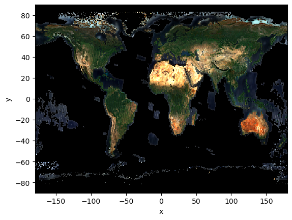
Notice that most of the ocean areas are coloured black (pixel value 0) instead of with a transparent colour. This is because cog3pio=0.1.0 doesn’t have the ability to deal with NaN values yet, so you will need to manually handle this.

Concatenate multiple single-band GeoTIFFs

Let’s now try a slightly trickier set up - with bands stored in different files!

We’ll use LandCoverNet images over Australia. Specifically, we’ll read multiple Sentinel-2 bands using xr.open_mfdataset, ensuring that the list of URLs/filepaths correspond to the band order we want.

Note that some parameters are different than before:

• concat_dim="band" and combine="nested": ensures that the bands are concatenated as data_vars along the dimension ‘band’

• device_id=None (actually the default setting): so that the data is decoded by whatever GPU is available (usually this is the first CUDA GPU device, unless you are using dask-cuda with multiple GPUs).

dataset: xr.Dataset = xr.open_mfdataset(
    paths=[
        "https://data.source.coop/radiantearth/landcovernet/landcovernet_au/data/v1.0/2018/56JMS/16/S2/56JMS_16_20180214/56JMS_16_20180214_B04_10m.tif",
        "https://data.source.coop/radiantearth/landcovernet/landcovernet_au/data/v1.0/2018/56JMS/16/S2/56JMS_16_20180214/56JMS_16_20180214_B03_10m.tif",
        "https://data.source.coop/radiantearth/landcovernet/landcovernet_au/data/v1.0/2018/56JMS/16/S2/56JMS_16_20180214/56JMS_16_20180214_B02_10m.tif",
    ],
    engine="cog3pio",
    concat_dim="band",
    combine="nested",
    device_id=None,
    parallel=True,
)
dataset

<xarray.Dataset> Size: 397kB
Dimensions:  (band: 3, y: 256, x: 256)
Coordinates:
  * band     (band) uint8 3B 0 0 0
  * y        (y) float64 2kB 7.187e+06 7.187e+06 ... 7.184e+06 7.184e+06
  * x        (x) float64 2kB 4.962e+05 4.962e+05 ... 4.988e+05 4.988e+05
Data variables:
    raster   (band, y, x) uint16 393kB dask.array<chunksize=(1, 256, 256), meta=np.ndarray>

xarray.Dataset

• Dimensions:
  • band: 3
  • y: 256
  • x: 256
• Coordinates: (3)
  • band
    (band)
    uint8
    0 0 0

    array([0, 0, 0], dtype=uint8)

  • y
    (y)
    float64
    7.187e+06 7.187e+06 ... 7.184e+06

    array([7186805., 7186795., 7186785., ..., 7184275., 7184265., 7184255.],
          shape=(256,))

  • x
    (x)
    float64
    4.962e+05 4.962e+05 ... 4.988e+05

    array([496225., 496235., 496245., ..., 498755., 498765., 498775.], shape=(256,))

• Data variables: (1)
  • raster
    (band, y, x)
    uint16
    dask.array<chunksize=(1, 256, 256), meta=np.ndarray>

    Array Chunk Bytes 384.00 kiB 128.00 kiB Shape (3, 256, 256) (1, 256, 256) Dask graph 3 chunks in 7 graph layers Data type uint16 numpy.ndarray

Next, we’ll retrieve the ‘raster’ xarray.DataArray data_var from the xarray.Dataset, and then call .load() to materialize the actual array into memory. This is because xr.open_mfdataset does lazy loading into Dask arrays by default, but we want CuPy arrays!

raster: xr.DataArray = dataset.raster.load() # TODO: needs patched xarray
# assert isinstance(raster.data, cp.ndarray) # TODO: dask loads into numpy, not cupy ☹️
raster

<xarray.DataArray 'raster' (band: 3, y: 256, x: 256)> Size: 393kB
array([[[ 395,  404,  412, ...,  423,  437,  481],
        [ 397,  412,  412, ...,  404,  456,  523],
        [ 398,  401,  408, ...,  420,  502,  560],
        ...,
        [ 360,  353,  361, ...,  373,  455,  457],
        [ 364,  361,  370, ...,  324,  376,  382],
        [ 372,  366,  370, ...,  339,  340,  356]],

       [[ 763,  743,  742, ...,  787,  824,  905],
        [ 729,  743,  761, ...,  787,  869,  963],
        [ 743,  746,  749, ...,  783,  895, 1005],
        ...,
        [ 715,  744,  753, ...,  507,  536,  508],
        [ 741,  736,  746, ...,  488,  520,  487],
        [ 741,  736,  744, ...,  479,  491,  487]],

       [[ 682,  689,  721, ...,  671,  700,  754],
        [ 695,  714,  703, ...,  675,  745,  781],
        [ 691,  711,  702, ...,  668,  754,  819],
        ...,
        [ 682,  696,  702, ...,  296,  332,  313],
        [ 697,  714,  689, ...,  288,  313,  280],
        [ 703,  700,  692, ...,  274,  283,  266]]],
      shape=(3, 256, 256), dtype=uint16)
Coordinates:
  * band     (band) uint8 3B 0 0 0
  * y        (y) float64 2kB 7.187e+06 7.187e+06 ... 7.184e+06 7.184e+06
  * x        (x) float64 2kB 4.962e+05 4.962e+05 ... 4.988e+05 4.988e+05

xarray.DataArray

'raster'

• band: 3
• y: 256
• x: 256

• 395 404 412 395 409 393 418 404 ... 313 424 416 298 294 274 283 266

  array([[[ 395,  404,  412, ...,  423,  437,  481],
          [ 397,  412,  412, ...,  404,  456,  523],
          [ 398,  401,  408, ...,  420,  502,  560],
          ...,
          [ 360,  353,  361, ...,  373,  455,  457],
          [ 364,  361,  370, ...,  324,  376,  382],
          [ 372,  366,  370, ...,  339,  340,  356]],
  
         [[ 763,  743,  742, ...,  787,  824,  905],
          [ 729,  743,  761, ...,  787,  869,  963],
          [ 743,  746,  749, ...,  783,  895, 1005],
          ...,
          [ 715,  744,  753, ...,  507,  536,  508],
          [ 741,  736,  746, ...,  488,  520,  487],
          [ 741,  736,  744, ...,  479,  491,  487]],
  
         [[ 682,  689,  721, ...,  671,  700,  754],
          [ 695,  714,  703, ...,  675,  745,  781],
          [ 691,  711,  702, ...,  668,  754,  819],
          ...,
          [ 682,  696,  702, ...,  296,  332,  313],
          [ 697,  714,  689, ...,  288,  313,  280],
          [ 703,  700,  692, ...,  274,  283,  266]]],
        shape=(3, 256, 256), dtype=uint16)

• Coordinates: (3)
  • band
    (band)
    uint8
    0 0 0

    array([0, 0, 0], dtype=uint8)

  • y
    (y)
    float64
    7.187e+06 7.187e+06 ... 7.184e+06

    array([7186805., 7186795., 7186785., ..., 7184275., 7184265., 7184255.],
          shape=(256,))

  • x
    (x)
    float64
    4.962e+05 4.962e+05 ... 4.988e+05

    array([496225., 496235., 496245., ..., 498755., 498765., 498775.], shape=(256,))

Finally, we’ll plot the RGB image. This is over a location at Hervey Bay, north of Sunshine Coast in Queensland, Australia.

raster.plot.imshow(robust=True)

<matplotlib.image.AxesImage at 0x7f740e25b9d0>

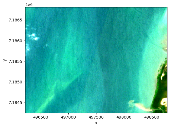
There’s some cloud to the left, mostly water in the middle, and a strip of land on the right. See if it matches with the label classifications here.

Summary

Awesome, you’ve now learned how to read GeoTIFFs into CUDA GPU memory, and uncovered some of the limitations such as no NaN handling and lack of support for certain compression types (TODO). This is a work in progress though, so feel free to open issues to contribute improvements if you’re keen to help!

See also

• Accelerating GeoTIFF readers with Rust - FOSS4G 2025 talk

• Decode GeoTIFF to GPU memory post on Pangeo forum

• GeoTIFF to GPU 3 part blog series